PD Dr. Stefan Immel - Atomic Orbitals

Atomic Orbitals

Although the Schrödinger equation may not be explicitly solved for many electron systems, DFT and ab initio calculations can be used to numerically and iteraviely solve the problem. Using this methodology, atomic and molecular orbitals can be computed, and the values of the wave functions or electron densities can be generated on three dimensional grids around atoms or molecules. This page gives an overview on some atomic orbitals calculated for "real" atoms. Orbitals were generated for the corresponding noble gases (n = 1: He, n = 1: Ne, n = 3: Ar, n = 4: Kr), with exception of the f-orbitals that were generated for the Luthetium (Lu). For more information on the Quantum numbers, and other orbitals of higher states (from the 1s up to the 6d level), see the hydrogenic orbitals generated for single electron systems (H, He⁺, Li²⁺, ...).

Calculations
Visualizations

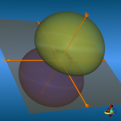
The following table provides an overview on the different types and shapes of orbitals from the 1s up to the 4f level. The orbitals are usually visualized as iso-contour surfaces on the electron density, thus a 90% probability surface displays the three-dimensional volume in which an electron is to be found with a 90% chance. Yellow and blue colors indicate regions of opposite sign of the wave function ψ (the electron density is proportional to ψ²); and the "nodal" planes indicate spatial areas (actually planes, spheres, and cones) were the wave function passes through zero and changes sign.

Lobes and Nodes of a 3p-Orbital

Atomic Orbitals - Calculations

In contrast to the hydrogenic orbitals generated from pure Cartesian wave functions, these images are for the "real" atoms, and all graphics were generated at a constant scale factor. Therefore, the size of the orbitals may be compared to each other for the different atoms (He, Ne, Ar, Kr, and Lu). Click on the individual images to obtain enlarged visualizations of the orbitals, respectively.

Atomic Orbitals - Visualizations

Quantum
Numbers